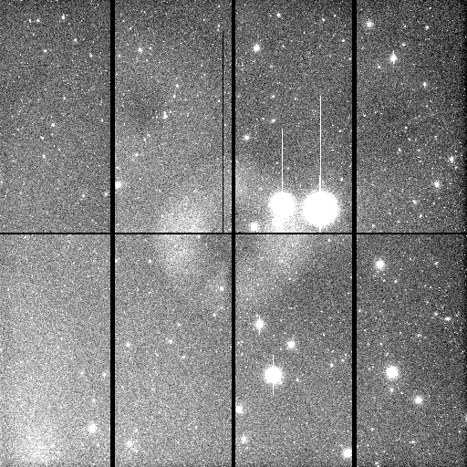
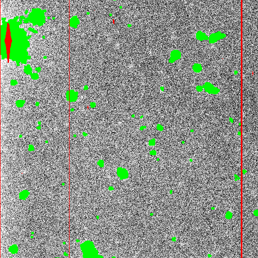
Figure 2: Example mosaic field.
Some new reduction capabilities were added in IRAF V2.12 and MSCRED V4.7. In this document we illustrate the capabilities with mosaic exposures the features may also be applied to single CCD images. The new features revolve around the creation and use of object masks for combining, pupil pattern removal, and fringe removal. The application to mosaic exposures is made more convenient by use of a new multiextension FITS file option for IRAF masks.
The next section presents an introduction to
the new multiextension FITS mask format and how it is used with IRAF tasks.
The following section introduces a key new mask
application, NPROTO.OBJMASKS, that produces object masks and sky maps for
various uses. One of these uses is for stacking images as discussed in
the section on combining . The final two sections
discuss the mosaic data reduction operations of pupil
pattern and fringe removal. The former is
mostly relevant to KPNO mosaic data. Whether pupil and fringe removal
are necessary depends on the filter. The new functionality is that these
two operations can now be reliably automated, whereas previously they
required interactive decisions by the user.
Multiextension FITS Masks
IRAF masks are files that identify a subset of image pixels with various integer values. These mask files may be used in the same way as images but are stored in a special format that is more compact than a regular raster image. Though may IRAF tasks don't currently make use of masks the number is growing.
Before IRAF V2.12 there was just one mask format. This is the pixel list format which is a special binary file with the extension ".pl". In V2.12 support was added for IRAF pixel masks in FITS binary table extensions based on one of the proposed conventions for FITS compressed image formats . The advantages of this for users are that these are valid FITS files and that these masks can be stored as extensions with other FITS data or multiple masks can be stored in a single file. This last capability is what is most useful for mosaic data reductions. This section provides a quick primer on creating and using this new mask capability in IRAF.
IRAF access to the FITS mask format is through the IRAF FITS kernel. This means that all the syntactical features of this kernel apply; in particular, how extension positions or extension names are specified, and how multiextensions files are built up using the append flag. These features are discussed in greater detail in the IRAF FITS Kernel User's Guide.
The new feature to the syntax is that if the qualifier "type=mask" is included in the kernel section when a mask is created, the FITS extension will be in the compact mask format. Note that since masks are stored as a binary tables and binary tables are always FITS extensions then mask files in this format are always multiextension files, even if there is only a single mask. The consequence of this is that the extension name (or extension number) will always be required.
When accessing a mask file the file extension (e.g. ".fits") is not needed unless there is another image file with the same root name but a different extension. Also the "type=mask" qualifier is only needed when creating a mask extension and is not needed with accessing an existing mask. Note that when the qualifier is used on the command line, a parameter query or in epar, the equal sign has to be escaped as shown in the examples of figure 1. The extension "pl" is just an example and any extension name may be used.
cl> imcopy def[pl] ghi[pl,type\=mask]
cl> imcopy def.pl ghi[pl,type\=mask]
cl> imstat ghi[pl]
cl> implot ghi[pl]
cl> display ghi[pl] 1 zs- zr- z1=-1 z2=2
cl> display obj 1 overlay=ghi[pl]
An object mask identifies pixels containing light from the astronomical objects in an image or mosaic. The complement is, naturally, the pixels which form the background. There are many data reduction steps which can benefit from separating the objects or the background. These include making sky flats and fringe templates and matching pupil and fringe patterns.
Object masks are created by applying an object detection algorithm. The most common algorithm consists of specifying or determining the image background and background noise and applying a threshold above the background to identify object pixels. For the purpose of creating a mask it is not really important to group pixels into objects, though detection algorithms do this. The IRAF Astronomical Cataloging Environment (ACE) package, which is under development, includes such an object detection algorithm.
While the complete ACE package is developed, the sky estimation, object detection, and mask creation task has been included in IRAF V2.12 in the NOAO prototype package, NPROTO. TO . The task is called OBJMASKS.
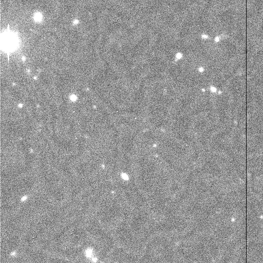
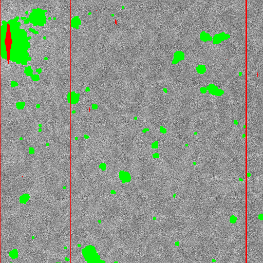
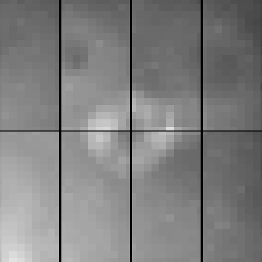
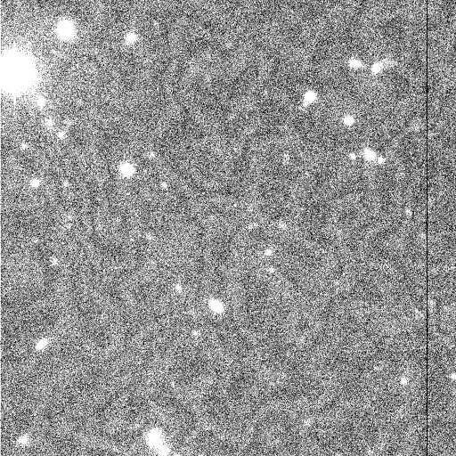
The help page describes the parameters and algorithms and gives some examples. Figure 2 shows an example mosaic image in which we will create an object mask and background sky map. A map is a reduced resolution image that is interpolated to the full size of the image to which it applies. The figure shows the full mosaic displayed at reduced resolution and a small region displayed at full resolution. The displays illustrate various features of this mosaic data; astronomical objects, a pupil pattern, fringing, variable sky background, and residual flat field patterns.
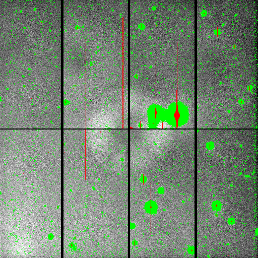
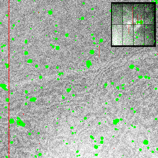
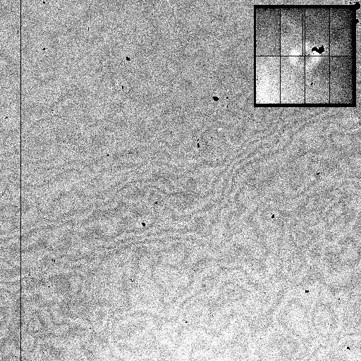
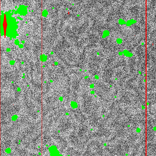
The commands in figure 3 create an object mask and sky map for all the extensions. Also shown is the command to display the object mask as an overlay on the mosaic image data (see figure 4 for the result). Note that the bad pixels are overlayed in red while the object pixels are in green. The last display command, which produces figure 5, illustrates how to display the sky maps as a mosaic.
ms> phelp objmasks
[output]
ms> objmasks obj262 om262 skys=sky262
[epar and output]
ms> mscdisplay obj262 1 over=!objmask ocolor="1-10=red,green"
[see figure 4]
ms> mscdisplay sky262 1 fill+
[see figure 5]
In addition to producing the object mask, OBJMASKS adds or modifies the image header keyword OBJMASK to record the object mask associated with the image. The header is only modified if the user has write permission on the input data. The OBJMASK keyword can then be referenced in tasks such as DISPLAY, MSCDISPLAY, IMCOMBINE, and COMBINE. Note that ability to reference keywords other than BPM in these tasks is new in IRAF V2.12 and MSCRED V4.7. Figure 6 shows the keyword and some display commands that use the object mask keyword.
ms> msccmd "imhead $input l+ | match OBJMASK" obj262
OBJMASK = 'om262[im1]'
OBJMASK = 'om262[im2]'
OBJMASK = 'om262[im3]'
OBJMASK = 'om262[im4]'
OBJMASK = 'om262[im5]'
OBJMASK = 'om262[im6]'
OBJMASK = 'om262[im7]'
OBJMASK = 'om262[im8]'
ms> display obj262[im2] 1 over=!objmask
ms> mscdisplay obj262 1 over=!objmask
ms> combine @list outcomb masktype=!objmask
A common image stacking operation is to combine only the sky or background pixels while excluding or rejecting the object pixels. This type of operation is used to create sky flat fields, pupil pattern templates, and fringe pattern templates. One way to do this is to apply a pixel rejection algorithm where the set of input pixels contributing to a combined output pixel are examined to find and reject statistically significant outliers. Sometimes additional pixels within some distance of the rejected pixels are also rejected.
The ability to create object masks provides another approach. The pixels identified in the object mask for each image contributing to the output combined pixels may be excluded without requiring a statistical test. The ability to use masks to exclude pixels has been in earlier versions of the primary combining tasks COMBINE and IMCOMBINE. What is new is that now it is fairly easy to generate the object masks with OBJMASKS.
In a sense the two methods are similar since the detection of the objects for the object mask is also a statistical outlier method. Some of the techniques of one could be incorporated into the other but the functionality would them be rather complex. The multiple image rejection methods primarily consider the statistics at a single pixel across multiple images while the object detection method considers the statistics of neighboring pixels in the same image.
In earlier versions of the IRAF COMBINE and IMCOMBINE tasks, the masks could only be assigned using the keyword BPM. A minor new feature of the combining tasks is that the "masktype" parameter may be specified as "!<keyword>", where <keyword> is any keyword whose value is the mask to be used. In this special case the good values in the mask are specified by the "maskval" parameter.
Figures 7 and 8 show the results of combining just two mosaic exposures of the same field with a small dither shift. In normal use there would be more exposures and they might be from a variety of fields. Object masks are first created for these two exposures using OBJMASKS as described previously. The combining is carried out as shown in figure 7. Because there are only two exposures in this example there are places where objects overlap. In this case the "blank" value is output. Figure 8 shows a region of each mosaic exposure with the object masks overlayed. The third display is of the combined exposure. The signal to noise ratio has been improved making the fringing and pupil pattern more visible. The black spots (which are hard to see in these figures) are the places where objects overlapped in the two exposures.
ms> combine obj262,obj263 comb masktype=!objmask scale=@scales
[epar and output]
ms> mscdisplay obj262 1 overlay=!objmask ocol="1-10=red,green"
[see figure 8]
ms> mscdisplay obj263 2 overlay=!objmask ocol="1-10=red,green"
[see figure 8]
ms> mscdisplay comb 3
[see figure 8]

A pupil pattern may be seen in KPNO Mosaic exposures at the Mayall telescope in certain filters. The data shown in the figures of this document have this pattern. The pattern is the ring feature in the center of the mosaic field. This pattern is seen in both the dome flat field and sky exposures. The pattern must be determined and then scaled and removed from this data. The dome flat fields are corrected by removing the pattern through division in order to preserve the underlying detector response pattern. The sky exposures are then corrected by the dome flat field. This leaves the pupil pattern in the sky exposures which is then removed by subtraction. This aspect of mosaic data reductions for KPNO Mosaic data has been described in various documents.
The problem has been that to obtain the best correction for either the dome flat field or sky exposures, the pupil pattern must be scaled interactively. In this section we present a new task which automates the scaling and removal of the pupil pattern.
The new task is RMPUPIL. Note that there was previously an interactive task by this name which is now called IRMFRINGE, where the "I" stands for interactive. The help page describes the parameters and algorithm.
The key to producing a reliable automatic scaling factor and correction is the use of object masks to isolate the pattern in the background from the contaminating objects. The masks are produced as shown in figure 3. When the pattern is relatively localized a sky map is not needed and would be compromised by the pupil pattern anyway. A second mask is also required which defines the regions in the pupil pattern template which are relevant.
The pupil pattern template is created by first making a sky flat from a set of exposures where the objects are dithered. Note that using object masks may improve the creation of the sky flat as described earlier. The same object masks may be used for the sky flat creation and the pupil scale fitting and removal. The pupil pattern is extracted from the sky flat using the task MSCPUPIL. These steps are described elsewhere. However, one new feature of MSCPUPIL is that it also generate a mask locating the pupil. This is shown in figures 9 and 10. Note that the pupil mask need be created only once and saved as a standard calibration file for all reductions.
ms> mscpupil obj262 Pupilmask type=mask
[epar and output]
ms> mscdisplay obj262 1 over=!objmask ocol="1-10=red,green"
[see figure 10]
ms> mscdisplay Pupil_I0421 2 over=Pupilmask
[see figure 10]
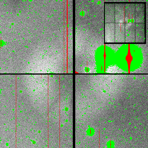
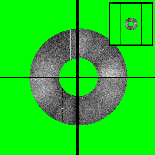
Figure 11 shows the commands and terminal output for running RMPUPIL and displaying the results as shown in figure 12. Since the pupil pattern only appears in the extensions im2, im3, im6, and im7 the extfit parameter is set to the extensions "im[2367]". In the log output the independent scale estimates for each extension are shown but the final scale is computed using all the fitting extensions. The single scale factor for the mosaic is then applied to create the pupil subtracted output.
ms> rmpupil obj262 pobj262 Pupil_I0421 om262
[epar and output]
ms> mscdisplay obj262 1 over=!objmask ocol="1-10=red,green"
[see figure 12]
ms> mscdisplay pobj262 2 over=!objmask ocol="1-10=red,green"
[see figure 12]

The correction applied by RMPUPIL is recorded in the correct output image header by the keyword RMPUPIL. Figure 13 shows these keywords in a mosaic exposure.
ms> msccmd "imhead $input l+ | match RMPUPIL" pobj262
RMPUPIL = 'obj262[im1] - 188.87 Pupil_I0421[im1]'
RMPUPIL = 'obj262[im2] - 188.87 Pupil_I0421[im2]'
RMPUPIL = 'obj262[im3] - 188.87 Pupil_I0421[im3]'
RMPUPIL = 'obj262[im4] - 188.87 Pupil_I0421[im4]'
RMPUPIL = 'obj262[im5] - 188.87 Pupil_I0421[im5]'
RMPUPIL = 'obj262[im6] - 188.87 Pupil_I0421[im6]'
RMPUPIL = 'obj262[im7] - 188.87 Pupil_I0421[im7]'
RMPUPIL = 'obj262[im8] - 188.87 Pupil_I0421[im8]'
The section describes how to remove fringing from mosaic data, though these same steps apply equally well to single images. Figure 14 shows a small region of one CCD in a mosaic exposure and the corresponding piece of the fringe pattern template. The basic steps for removing fringing are creating a template of the fringe pattern, creating a mask that isolates the background in each exposure, creating a background map when there are background gradients across the exposure, determining the scale factor that best matches the fringe template to the exposure, and subtracting the scaled fringe template from the exposure.

A fringe template is constructed from all the sky exposures which exhibit the same fringe pattern. The best result is obtained using dark sky exposures where the fields have been dithered so that every pixel has several exposures that are uncontaminated by sources. The exposures are put together to make a fringe template using the COMBINE task. The images are scaled to a common level and objects are excluded by rejection and masking techniques. Descriptions of how this is done using rejection algorithms are given elsewhere. However, use of OBJMASKS to create object masks to be excluded during combining is a new capability that can be used. Note that making object masks (and background maps) for each exposure is needed for automatic computation and removal of the fringing so making the masks for creating the fringe template does not add unnecessary processing.
One step in the creation of the fringe template recommended in other descriptions is the removal of the background on scales greater than the fringe pattern. This is done with surface fitting or median/average block filtering using large box sizes. The way the fringe template is fit to the observations computes and corrects for any mean value. So there is no need to make the mean of the fringe template be zero though background structure in the fringe template, such as gradients of large scale undulations, do need to be removed.
One might wonder whether object masks created for pupil pattern removal might not be used for the fringe removal. The objects detected will be the same in the data which is not contaminated by the pupil pattern. In the KPNO mosaic this is the case for four of the eight CCDs. And where the pattern is present the objects will not change very much. So it is likely that these would work fine. The main concern is that when the exposures exhibit background gradients the sky maps produced when the objects are detected will be affected by the pupil pattern. Even so this may not significantly affect the quality of the fringe scale determination. It is also possible to use only those extensions not affected by the pupil pattern for estimating the the fringe scaling. So it is quite possible that creating the object masks again is not necessary. But in this section we describe creating the object masks and sky maps and applying these in the fringe scale determination using all the extensions in the pupil pattern corrected data.
The object masks and sky background maps used for the fringe removal (and possibly for the fringe frame creation) are created using the task OBJMASKS. Figure 15 shows the commands to create these files for a single mosaic exposure and to display the sky background as shown in figure 16. The mosaic exposure is the same one used to illustrate the pupil pattern removal in the previous section. In this case the pupil pattern corrected data is used. So the sky map shown in figure 16 is similar to figure 5 except the pupil pattern is no longer evident. This sky shows a gradient as well as some flat field patterns to be removed in a final sky flat field correction. Note that the sky map is only needed if there is a significant sky gradient. The mean sky level is automatically accounted for during the fringe removal step.
ms> objmasks pobj262 om262 skys=sky262
[epar and output]
ms> mscdisplay sky262 1 fill+
[see figure 16]
The object masks and sky maps produced by OBJMASKS are used in the task RMFRINGE to automatically determine the fringe scaling and subtract the pattern. There in MSCRED versions before V4.7 the task RMFRINGE was a different program that required interactively displaying and entering scaling factors until the pattern was removed to the satisfaction of the user. This previous task is now called IRMFRINGE and the new version of RMFRINGE is an automatic pattern fitting algorithm.
Figure 17 shows the parameters, execution, and output from RMFRINGE. The commands to produce the displays in figure 18 are also shown. It is difficult to see the details in that figure but the fringing is well removed. In this example all the extensions are used to determine the global fringe scale factor for the mosaic exposure. As mentioned earlier, the parameter "extfit" could be used to select a subset of extension and the object mask and sky maps would only be needed for those extensions. However, the fringe pattern template must be created for all the extensions and the output contains all the extensions.
ms> rmfringe pobj262 pfobj262 FringeI010421 om262 back=sky262
[epar and output]
ms> display pobj262[im2] 1 over=!objmask ocol="1-10=red,green"
[see figure 18]
ms> display pfobj262[im2] 2 over=!objmask ocol="1-10=red,green"
[see figure 18]
One feature that that can be seen in figure 18 is a brightening of background on the left edge. The section shown is on the edge of the second CCD in the mosaic. The brightening is caused a drop in the fringe pattern at the edge which can be seen in figure 14. This artifact was produced during the background removal when creating the fringe pattern template.
The correction applied by RMPUPIL is recorded in the correct output image header by the keyword RMPUPIL. Figure 19 shows these keywords in a mosaic exposure.
ms> msccmd "imhead $input l+ | match RMFRINGE" pfobj262
RMFRINGE= 'pobj262[im1] - 0.81727 (FringeI010421[im1] - 0.49265)'
RMFRINGE= 'pobj262[im2] - 0.81727 (FringeI010421[im2] - 0.49265)'
RMFRINGE= 'pobj262[im3] - 0.81727 (FringeI010421[im3] - 0.49265)'
RMFRINGE= 'pobj262[im4] - 0.81727 (FringeI010421[im4] - 0.49265)'
RMFRINGE= 'pobj262[im5] - 0.81727 (FringeI010421[im5] - 0.49265)'
RMFRINGE= 'pobj262[im6] - 0.81727 (FringeI010421[im6] - 0.49265)'
RMFRINGE= 'pobj262[im7] - 0.81727 (FringeI010421[im7] - 0.49265)'
RMFRINGE= 'pobj262[im8] - 0.81727 (FringeI010421[im8] - 0.49265)'